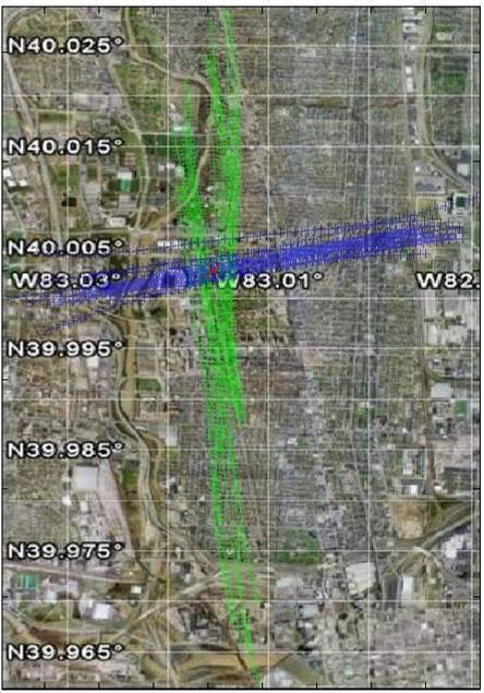
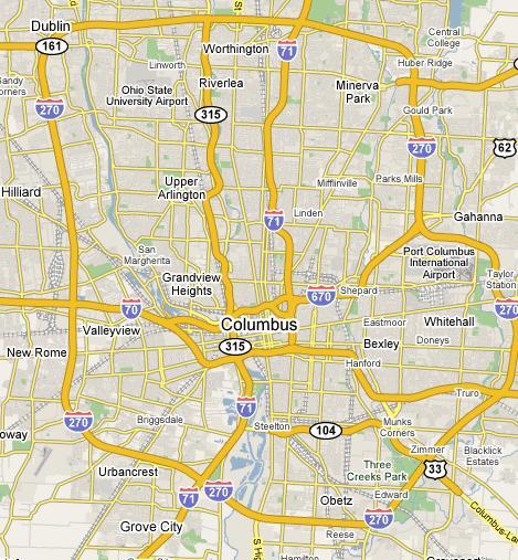
The Columbus Surrogate Unmanned Aerial Vehicle (CSUAV) data collection consisted of two surrogate UAV platforms flying a dog bone course centered over the campus of The Ohio State University. The data collection occurred on October 28, 2007 between 11:00 am and 1:21 pm local time. A total of fifteen runs were executed, where each run is defined as a continuous sensor data recording over a linear portion of the dog bone course. Each CSUAV platform flew nominally at a constant altitude and carried a single sensor payload with an approximate nadir view angle for the duration of the data collection. The two sensor payloads were an Illunis XMV-11000 EO (monochrome CCD) visible camera and a FLIR Systems ThermoVision SC6000 MWIR (3-5 µm) camera. The CSUAV EO and MWIR platforms flew nominally E—W and N—S coincident runs, respectively. The image in Figure 1 depicts the sensor ground tracks for each run over a Google Earth image, while the image in Figure 2 depicts the notional ground tracks over a map for reference. In both images, the blue lines represent the EO platform ground tracks while the green lines represent the MWIR platform. The planned ground track intersection point is east of Ohio Stadium at the intersection of Neil Avenue and West 19th Avenue.
The sensor parameters for the CSUAV platforms are listed in Table 1. The EO platform flew nominally at a 6.5 kft. altitude (MSL) while the MWIR platform flew at a 2.5 kft. altitude (MSL). The EO platform air speed varied between 90 and 130 knots over the duration of the data collection while the MWIR platform air speed was between 80 and 100 knots. In both cases, the air speed within an individual run remained relatively constant compared to the air speed across runs. The EO platform collected between 234 and 329 frames per run while the MWIR platform collected between 2087 and 3723 frames per run. Given the parameters in Table 1 and the nominal platform altitudes, the spatial resolution for the EO sensor is 0.61 x 0.61 ft./pixel while the spatial resolution for the MWIR sensor is 0.88 x 0.88 ft./pixel.
| Sensor |
Frame Size (H x V) |
FOV (H° x V°) |
Focal Length (mm) |
FPA Pixel Pitch (µm) |
Frame Rate (Hz) |
Dynamic Range |
|---|---|---|---|---|---|---|
| Illunix XMV-11000 |
4004 x 2672 |
23.9° x 16.1° |
85 |
9 x 9 |
~5 |
12 bits |
| FLIR Systems ThermoVision SC6000 |
640 x 512 |
18.2° x 14.6° |
50 |
25 x 25 |
30 |
14 bits |
There are two AVIs included that contain all of the frames from run 1 per sensor. They are encoded with the Microsoft MPEG-4 version 2 codec at 5 frames per second (EO) and 30 frames per second (IR), respectively. The AVIs contain the raw filename, time stamp (local time) and frame number in the top left corner of each frame. Equalization of the raw frame was performed for image enhancement on both AVIs.
Matlab m-files are provided that read and view the raw data files as described below.